1.4 Central Tendency and Variability
Objective
A probability distribution (or "distribution" for short) describes the possible outcomes for an event, and how likely each of those outcomes are. When characterizing a distribution of categorical or quantitative values, the things you typically want to know are: 1) where's the center, 2) how fat or thin is it, and 3) does it have any unusual characteristics (e.g. is it skewed to the right or left, does it have more than one hump, is it asymmetric). "Central tendency" is a fancy sounding phrase that just means: if you have a whole bunch of values, where is the middle of all those values (and what does "middle" even mean)? Measures of variability (e.g. variance and standard deviation) tell you how fat or thin your distribution is. This chapter covers these two basic topics, including how to compute them analytically and how to compute them in R. Distribution shapes are covered in the chapter on histograms.
Who cares about such a simple topic? Well, just knowing the values for the mean, median, and mode, coupled with the variability information provided by the variance and standard deviation, you can get a sense of the shape of your distribution. You can also sometimes get a sense for what proportion of your observations fall within various bounds. Also, many of the statistical inference tests you perform are related to figuring out if you really know where the center of a particular distribution is located. If you read fancy proofs, you'll hear the term "Expected Value" quite a lot. What they mean is: the value we think is in the middle of all the possibilities. That's all. This chapter covers the first two of these basic topics, including how to compute them analytically and how to compute them in R. Distribution shapes are covered in the chapter on histograms.
Mean (Arithmetic)
The arithmetic mean identifies the midpoint between all the values in a dataset of numbers, even if there isn't an observed value at the midpoint. It is calculated by adding up all of the values, then dividing by the total number of observations. Finding a mean in R is simple, because you can pass values directly to mean or give it a vector or data frame selection:
The arithmetic mean is not the only variety of mean that can be used to express central tendency! The geometric mean and harmonic mean are also potential measures if your quantitative data is on the ratio level of measurement (and, for the geometric mean, if your values are positive). The geometric mean characterizes the average growth rate between values, and is often used in financial applications. The harmonic mean characterizes an average rate. I've never used the geometric or harmonic means for data analysis personally, though, so I can't provide any recommendations beyond noting that you can potentially use these.
Median
The median identifies the observation that sits at the midpoint between all the observations in a dataset. If there are an even number of observations, the median is computed as the arithmetic mean of those two observations that sit at the midpoint. Like mean, you can pass values directly to median or give it a vector or data frame selection. Here are some examples in R:
As long as the values in a dataset can be ordered, you can find the one (or two) observations that sit at the midpoint, and thus find the median. You can compute a median for all kinds of variables... except categorical variables that are nominal. As an example, you can't compute the median of several M&M colors (because that's a categorical variable at the nominal level of measurement) but you can compute the median of several scrabble tile values (because those letters can be ordered). Because of its versatility, there are many inference tests that can be done to compare the medians of datasets.
Mode
The mode identifies the most frequently observed value in a dataset. Unlike the median, calculation of the mode is not precluded by the level of measurement. For example, it's possible to determine:
The mode of M&M colors in a bag (that is, the most frequently observed color)
The mode of Scrabble tiles still left in the bag (that is, the letter or letters that have the most tiles available)
The mode of customer satisfaction responses (that is, which item between "Strongly Dissatisfied" and "Strongly Satisfied" was most frequently selected)
The mode for daily high temperatures in summer (that is, which high temperature occurs most frequently)
These illustrate what the mode looks and feels like for nominal, ordinal, interval, and ratio level data, respectively. The only one you have to be careful with are modes for ratio level quantitative variables, because sometimes the mode is just not meaningful. As an example, think about what your data might look like if you're measuring how much people weigh. If you're collecting that data in pounds to the second decimal place, it's likely that your data looks something like this, with no repeated values:
145.59 220.31 197.63 105.25 118.80 145.14 170.28 166.37
It would be really unlikely for the mode to be meaningful in this case: we might not have any numbers that are observed more than once, making the "most frequently appearing observation" absurd. Bottom line: if you have ratio level data, check to make sure the mode is meaningful before you report it. It's actually pretty easy with R to determine if a mode is "meaningful" or not. Here's an example where the mode is clearly meaningful. First, we pull 100 random numbers from a uniform distribution between 1 and 10. (This is just like rolling dice, only we're working with a 10-sided die where each of the numbers 1 through 10 is equally likely to appear. That's the purpose of the runif function.)
Now, let's add up how many 1's, 2's, 3's and so forth we got using the random number generator by invoking the table command. The top row represents the numbers from 1 to 10, and the bottom row includes the counts of how many of those random numbers were generated by runif. Using sort arranges the numbers so that the lowest frequencies appear first, and the higher frequencies appear later.
Here are the commands we can use to pull out which elements of x appear most frequently (mode.names) and how many times they appear (max(y)). As long as you store your sorted table in a variable called y, you will be able to use these commands to identify the mode (or modes, because you can have more than one) and the observation count that corresponds to that maximum value.
This also works if your values are categorical (at the nominal level of measurement). Imagine that you own a restaurant specializing in New Mexican cuisine. You want to find out how your customers prefer the chile on their burritos: red, green, or Christmas. Here's a way to simulate that data from 100 customers:
The mode can be determined the same way as in the previous example:
What about the case where the mode is meaningless? Well, that's what would have happened if we didn't round our randomly sampled numbers between 1 and 10. Try this, and you'll see a mode that's not meaningful at all:
What's the frequency of our mode? One. Just one observation. That means EVERY SINGLE ONE of the values we generated is the mode. A hundred values, a hundred modes. If everyone is an important mode, then no one is an important mode. The mode, in this case, is meaningless as an indicator of central tendency.
Relationships Between Mean, Median, & Mode
If you have a collection of quantitative values, and you know the mean, median, and mode, there are a lot of things you can figure out about the shape of your distribution. As a result, these measures of central tendency are like clues that you can use to draw a picture of the distribution in your head:
The mode is always at the highest point of the distribution... the peak.
If the distribution is skewed to the left, meaning that it has a tail stretching out along the left side of the x-axis... the median is pulled to the left.
If the distribution is skewed to the left, the mean is also pulled to the left. But all it takes is one or two outliers to really really pull that mean even farther to the left. The mean is much more sensitive to outliers than the median.
If the distribution is skewed to the right, meaning that it has a tail stretching out along the right side of the x-axis... the median is pulled to the right.
If the distribution is skewed to the right, the mean is also pulled to the right. But all it takes is one or two outliers to really really pull that mean even farther to the right. The mean is much more sensitive to outliers than the median.
In a symmetric distribution like the normal, the mean, median, and mode are all lined up together at the peak of the distribution. The most frequently observed value (mode) is the same as the average value (mean). Exactly 50% of the observations are below the mean, and 50% of the observations are above the mean, putting the median at the same spot as the mean.
In summary, here are the measures of central tendency that can be applied to the various variable types and levels of measurement:
| Variable Type | Level of Measurement | Ways to Represent Central Tendency |
|---|---|---|
| Categorical | Nominal | Mode |
| Ordinal | Median | |
| Quantitative | Interval | Arithmetic Mean, Median, Mode |
| Ratio | Arithmetic Mean, Median, Mode, Geometric Mean, Harmonic Mean |
Variance
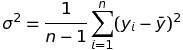
The variance represents how spread apart the values in your distribution are, and as a result, characterizes how fat or thin the distribution will be when plotted. To get the variance, you need to know all of the values in your dataset. You use them to calculate variance like this:
First, find the arithmetic mean of all the values.
Find the squared deviations: Take each value one at a time, and subtract the mean (which gives you negative numbers for all values that are below the mean, and positive numbers for all values that are above the mean) and then square whatever you get (that is, multiply it by itself). This makes all the values positive.
Now divide the total of all those squared deviations you just figured out by one less than the number of observations. (Why don't we just use the actual number of observations, and take the average? Because that would be biased... but more on that later when we talk about Bessel's correction.)
The equation that represents variance looks like this. Variance is represented by σ2, and n is the number of observations. The sum is over all elements of your dataset (from the first one through the nth one), and you're adding up the squared differences between each value and the overall mean:
Variance is also very easy to figure out in R, as long as you have your data arranged in a vector (or can extract a vector out of a data frame). For simplicity, let's use the values that are stored in x - the ones we got from sampling 100 random numbers between 1 and 10:
Take the square root of the variance, and you'll get the standard deviation:
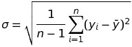
This is also dead easy to do in R using the sd command. Of course, if you have the variance handy, you can just take the square root of that to get the standard deviation and it all works out the same:
Bessel's Correction: Why We Divide by (n-1)
If you Google around to find equations for calculating the variance and standard deviation, sometimes they tell you to divide by the total number of observations n, and other times they tell you to divide by (n-1). Oh no!! Which one should you believe? What do you do? And which one does R do?
Which one should you believe? Believe the (n-1) version. It's more accurate, especially when the sample size is small.
What do you choose when you have to calculate it yourself? If you calculate variance and standard deviation yourself, be sure to use the (n-1) version.
Which one does R use? Fortunately, R uses the (n-1) version for both the variance and the standard deviation... so you can trust R.
What's the Rationale for Bessel's Correction?
The smaller your sample, the less likely you are to realistically capture the magnitude of the variance in a distribution. It takes a lot of observations to get a good sense of the true spread-outed-ness of values within a distribution!
But to determine the variance and standard deviation, you have to know the mean of the entire population (or at least have a good idea what it is). You're only guaranteed to estimate this well if you have a really big sample. So with an ordinary sized sample, you're not going to capture all of the variance that's really there. You need to bump up your estimate to account for the variability that you can't see. And since this is always true for sample sizes that are 2 or more...

...that means if you use the (n-1) version, you'll be making your estimates of the variance and standard deviation just a little bigger. The bigger the sample size n gets, the closer the biased estimator (where you divide by n) will be to the unbiased estimator (where you divide by n-1). Unbiased is better. This adjustment improves your variance estimate tremendously, and your standard deviation estimate almost as tremendously.
Other Resources
Did you know there are guidelines on how to report central tendency and variability in APA style research papers? Details are provided here: http://statistics-help-for-students.com/How_do_I_report_central_tendency_and_dispersion_data_in_APA_style.htm#.VQtgtI7F-o0
Find out more about Bessel's correction (n-1 in the calculation of the variance and standard deviation) at http://en.wikipedia.org/wiki/Bessel%27s_correction
A really nice, intuitive explanation for Bessel's correction with graphs is here: http://www.physics.ohio-state.edu/~durkin/phys416/Fall2011/LectureExtras/besselfactor.pdf