2.10 Contingency Tables/Marginal & Conditional Distributions
Objective
Contingency tables display the frequencies and relative frequencies of observations, which are classified according to two categorical variables. The elements of one category are displayed across the columns; the elements of the other category are displayed over the rows. This chapter shows you how to draw simple contingency tables, and more complex (beautiful) contingency tables! Fortunately, it is just as easy to create both kinds in R.
Simple Contingency Tables with table
There is already a built-in function in base R to construct contingency tables. To see this in action, let's load in M&M data representing 1922 individual M&M candies:
Check to make sure the data has loaded correctly:
# A tibble: 1,922 x 7
student id color defect full.bag.weight empty.bag.weight total.number
<chr> <int> <chr> <chr> <dbl> <dbl> <int>
1 alborb 1 R N 49.4 1.02 55
2 alborb 2 BR L 49.4 1.02 55
3 alborb 3 G N 49.4 1.02 55
4 alborb 4 R C 49.4 1.02 55
5 alborb 5 R N 49.4 1.02 55
6 alborb 6 BL N 49.4 1.02 55
7 alborb 7 R L 49.4 1.02 55
8 alborb 8 BL N 49.4 1.02 55
9 alborb 9 R L 49.4 1.02 55
10 alborb 10 R M 49.4 1.02 55
# ... with 1,912 more rows
Now you can create a contingency table using the table command from base R. The first argument points to the categorical variable that will appear over the rows, and the second argument indicates which categorical variable you want to span the columns:
C L M N
BL 10 96 7 198
BR 7 82 7 144
G 10 115 13 237
O 26 115 11 268
R 22 72 18 207
Y 17 76 7 157
More Fancy Contingency Tables with CrossTable
Since your data is already loaded into R and stored in the mnms object, it is easy to make an even more beautiful contingency table by using CrossTable in the gmodels package. Before you start, be sure to install the new package using install.packages("gmodels") and call its functions into active memory using library(gmodels).
The simplest contingency table is actually prepared using lots of arguments to CrossTable, where we have to turn off several of the features (don't worry, we'll turn them on later in this chapter). In contrast to the simple display produced by table, this one contains the row totals in the rightmost margin, and the column totals on the bottom margin.
Total Observations in Table: 1922
| mnms$defect
mnms$color | C | L | M | N | Row Total |
-------------|-----------|-----------|-----------|-----------|-----------|
BL | 10 | 96 | 7 | 198 | 311 |
-------------|-----------|-----------|-----------|-----------|-----------|
BR | 7 | 82 | 7 | 144 | 240 |
-------------|-----------|-----------|-----------|-----------|-----------|
G | 10 | 115 | 13 | 237 | 375 |
-------------|-----------|-----------|-----------|-----------|-----------|
O | 26 | 115 | 11 | 268 | 420 |
-------------|-----------|-----------|-----------|-----------|-----------|
R | 22 | 72 | 18 | 207 | 319 |
-------------|-----------|-----------|-----------|-----------|-----------|
Y | 17 | 76 | 7 | 157 | 257 |
-------------|-----------|-----------|-----------|-----------|-----------|
Column Total | 92 | 556 | 63 | 1211 | 1922 |
-------------|-----------|-----------|-----------|-----------|-----------|
If you store the output from CrossTable to a variable (I’ll call it m) you can get frequencies (with m$t), row proportions (with m$prop.row), column proportions (with m$prop.col), and table proportions (with m$prop.tbl). Each row adds up to 100% with m$prop.row, and each column adds up to 100% with m$prop.col. A full example appears on p. 154.
x C L M N
BL 0.03215434 0.30868167 0.02250804 0.63665595
BR 0.02916667 0.34166667 0.02916667 0.60000000
G 0.02666667 0.30666667 0.03466667 0.63200000
O 0.06190476 0.27380952 0.02619048 0.63809524
R 0.06896552 0.22570533 0.05642633 0.64890282
Y 0.06614786 0.29571984 0.02723735 0.61089494
x C L M N
BL 0.11 0.17 0.11 0.16
BR 0.08 0.15 0.11 0.12
G 0.11 0.21 0.21 0.20
O 0.28 0.21 0.17 0.22
R 0.24 0.13 0.29 0.17
Y 0.18 0.14 0.11 0.13| Chi-square contribution |
| N / Row Total |
| N / Col Total |
| N / Table Total |
|-------------------------|
Total Observations in Table: 1922
| mnms$defect
mnms$color | C | L | M | N | Row Total |
-------------|-----------|-----------|-----------|-----------|-----------|
BL | 10 | 96 | 7 | 198 | 311 |
| 1.604 | 0.405 | 1.001 | 0.021 | |
| 0.032 | 0.309 | 0.023 | 0.637 | 0.162 |
| 0.109 | 0.173 | 0.111 | 0.164 | |
| 0.005 | 0.050 | 0.004 | 0.103 | |
-------------|-----------|-----------|-----------|-----------|-----------|
BR | 7 | 82 | 7 | 144 | 240 |
| 1.753 | 2.277 | 0.096 | 0.344 | |
| 0.029 | 0.342 | 0.029 | 0.600 | 0.125 |
| 0.076 | 0.147 | 0.111 | 0.119 | |
| 0.004 | 0.043 | 0.004 | 0.075 | |
-------------|-----------|-----------|-----------|-----------|-----------|
G | 10 | 115 | 13 | 237 | 375 |
| 3.521 | 0.392 | 0.041 | 0.002 | |
| 0.027 | 0.307 | 0.035 | 0.632 | 0.195 |
| 0.109 | 0.207 | 0.206 | 0.196 | |
| 0.005 | 0.060 | 0.007 | 0.123 | |
-------------|-----------|-----------|-----------|-----------|-----------|
O | 26 | 115 | 11 | 268 | 420 |
| 1.729 | 0.348 | 0.556 | 0.043 | |
| 0.062 | 0.274 | 0.026 | 0.638 | 0.219 |
| 0.283 | 0.207 | 0.175 | 0.221 | |
| 0.014 | 0.060 | 0.006 | 0.139 | |
-------------|-----------|-----------|-----------|-----------|-----------|
R | 22 | 72 | 18 | 207 | 319 |
| 2.967 | 4.457 | 5.442 | 0.180 | |
| 0.069 | 0.226 | 0.056 | 0.649 | 0.166 |
| 0.239 | 0.129 | 0.286 | 0.171 | |
| 0.011 | 0.037 | 0.009 | 0.108 | |
-------------|-----------|-----------|-----------|-----------|-----------|
Y | 17 | 76 | 7 | 157 | 257 |
| 1.794 | 0.037 | 0.241 | 0.150 | |
| 0.066 | 0.296 | 0.027 | 0.611 | 0.134 |
| 0.185 | 0.137 | 0.111 | 0.130 | |
| 0.009 | 0.040 | 0.004 | 0.082 | |
-------------|-----------|-----------|-----------|-----------|-----------|
Column Total | 92 | 556 | 63 | 1211 | 1922 |
| 0.048 | 0.289 | 0.033 | 0.630 | |
-------------|-----------|-----------|-----------|-----------|-----------|
If you set the chisq argument to TRUE, this will also appear below your table:
Statistics for All Table Factors
Pearson's Chi-squared test
------------------------------------------------------------
Chi^2 = 29.40006 d.f. = 15 p = 0.0142785
With a p-value that's so low (anything above 0.05 is considered "high"), we reject the null hypothesis of the Chi-square test of independence, which is that the two categorical variables are independent of one another. There appears to be a relationship between the color of the M&M, and whether or not it has defects, based on this data set.
Here is a summary of some arguments you can pass to CrossTable:
| Aspect of Experiment | Description |
|---|---|
| prop.t | When set to TRUE, the number of observations in each cell divided by the total number of observations in the entire contingency table will be reported. |
| prop.r | When set to TRUE, the number of observations in each cell divided by the total number of observations in the row will be reported. |
| prop.c | When set to TRUE, the number of observations in each cell divided by the total number of observations in the column will be reported. |
| chisq | When set to TRUE, a Chi-square test of independence will be conducted on your data, and the value of the test statistic χ2 and the P-Value will be reported. |
| prop.chisq | When set to TRUE, the contribution of each cell to the test statistic χ2 will be reported. (Add up all of these values within the contingency table, and you should get the value of the reported χ2). |
| expected | When set to TRUE, this value will include the frequencies that each cell will have IF the two categorical variables are independent of one another. (This is extremely useful if you are performing a Chi-square test of independence analytically, using the formula for computing χ2). |
Marginal Distributions
Embedded within each contingency table, there are exactly two marginal distributions: one for each of the total observed frequencies for each of the two categorical variables. They are called marginal distributions because they include the totals displayed on the edges (or margins) of the contingency table: the row totals on the rightmost margin, and the column totals on the bottom margin. With the M&M data, that means:
There is one marginal distribution of colors. We can produce a barplot with the frequencies or relative frequencies of the colors – independent of defects.
There is one marginal distribution of defects. Our barplot can show the frequencies or relative frequencies of all the defects that we observed – independent of color.
Embedded within each contingency table, there are also many conditional distributions: that is, how frequently one of the categorical variables is observed given that you specifically set the other categorical variable to equal a specific value. Because you're setting a condition that one of the categorical variables has a specific value, each distributions is called conditional. Here are all the conditional distributions you can produce from the M&M data:
The distribution of colors for all M&Ms that are Chipped or Cracked
The distribution of colors for all M&Ms that have Letter defects
The distribution of colors for all M&Ms that have Multiple defects
The distribution of colors for all M&Ms that have No defects
The distribution of defects over all the Blue M&Ms
The distribution of defects over all the BRown M&Ms
The distribution of defects over all the Green M&Ms
The distribution of defects over all the Orange M&Ms
The distribution of defects over all the Red M&Ms
The distribution of defects over all the Yellow M&Ms
On the left we see the distribution of defects for all green M&Ms, and on the right, we see the distribution of colors for all chipped or cracked M&Ms:
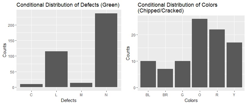
The code that produced the barplots above first requires that you filter out the information that is contained in the contingency table. For the leftmost plot, that means this:
[mnms %>% filter(color=="G") %>% group_by(defect) %>%
tally()]{.underline}
# A tibble: 4 x 2
defect n
<chr> <int>
1 C 10
2 L 115
3 M 13
4 N 237This can be embedded within a functional sequence that generates the plots:
Now What?
Find out more information about CrossTable at http://www.inside-r.org/node/89238
I also found this fantastic paper that describes how one researcher is exploring alternative (and hopefully better!) ways to visualize categorical data. In addition to being an interesting read, it demonstrates alternatives like the mosaic: http://www.datavis.ca/papers/koln/kolnpapr.pdf
The vcd and vcdExtra packages provide more sophisticated ways to display categorical data: http://www.datavis.ca/courses/VCD/vcd-tutorial.pdf