1.7 PDFs and CDFs
When an outcome is random, how do you mathematically describe the scope of all possibilities? You can do this by characterizing the distribution of all those possibilities as a probability density function (PDF). For discrete variables, it’s called a probability mass function (PMF). The PDF illustrates: how frequently do you observe certain values? The cumulative distribution function (or CDF) complements the PDF, and provides additional information. It shows what proportion of all observations will be less than or equal to a certain value. When you think of the normal distribution as a bell curve, you're thinking about the PDF.
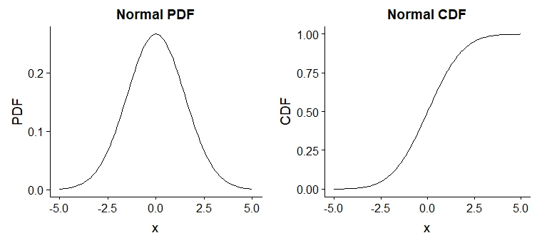
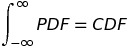
A probability density just tells you, for any given x-value, the long-run relative frequency of seeing a particular outcome occur. The CDF is the integral of the PDF:
Because integration means to add up all the areas underneath a function, we can think about it this way. Pretend you are a tiny person standing in front of a bell curve that looks like the normal PDF. You and the normal PDF are on a stage, and there's a stage curtain hanging on rings along the top edge of the stage. We're going to start at x=-4 and walk along the x-axis towards the right, all the way to x=+4. As we do, we're going to hold the curtain and pull it as we walk. How much of the area under the normal PDF are we covering as we walk by? Let's visually integrate to construct the CDF:
When you just start walking, and you go from x=-4 to x=-2, you're only capturing a tiny bit of the area under the normal PDF. The y-values on the CDF start at 0, because you have not covered any of the area under the normal PDF yet. The y-value at x=-2 will be about 0.16, since that's how much area we have covered by the time we have walked to x=-2.
As you walk from x=-2 to x=0, you're capturing the area at a faster and faster rate. By the time you get to x=0, you have captured 50% of the area under the normal PDF. The slope on the normal CDF thus increases to reflect that we're capturing the area faster. The y-value of the normal CDF at x=0 is 0.5, to reflect that we have captured half the area.
As we keep walking to the right, from x=0 to x=+2, we are capturing area at a slower rate. The slope of the CDF begins to decrease. When we get to x=+2, the y-value on the CDF will be 0.84, reflecting that we have covered 84% of the area under the normal PDF by this point.
Finally, as we walk from x=+2 to x=+4, we are adding area at a much, much slower rate. The slope on the normal CDF decreases to reflect that. By the time we've walked all the way across the stage, we have covered 100% of the area under the normal PDF, and the y-value on the normal CDF levels off at 1.0.
The probability density function, then, represents the rate of change of the cumulative distribution. It is the derivative of the CDF. If you know the equation of either the PDF or the CDF, you can determine the equation for the other function by integrating or differentiating, respectively.
You can visually differentiate a CDF by pretending you're a tiny person walking from the leftmost position on the x-axis to the rightmost position. All you have to do to create a PDF is to eyeball the slope of the CDF, and plot that value on the y-axis of the PDF you are creating. The area under a PDF is, by definition, 1. The range of values on the y-axis of the CDF is always 0.0 to 1.0. This is a very convenient property that enables us to create inverse transform equations to generate random numbers from any target distribution we want. Fortunately, there are several functions built into R which make it super easy to work with PDFs and CDFs. All you need to know is the value of the parameters that uniquely specify any given distribution. The normal distribution is fully specified by its mean (which shows where the center of the distribution is at) and standard deviation (which shows how spread out the values are).
| R Command | What it does |
|---|---|
| rnorm(n,mean,sd) | Generates n random variates selected from a normal distribution with specified mean and standard deviation |
| dnorm(x,mean,sd) | Plots the PDF from a collection of values x (which represent various points along the x-axis) centered at the specified mean, and with the specified standard deviation |
| pnorm(x,mean,sd) | Plots the CDF from a collection of values x (which represent various points along the x-axis) centered at the specified mean, and with the specified standard deviation |
| qnorm(area,mean,sd) | Finds the quantiles, or Inverse CDF. If you know an area under the normal PDF to the left of a particular x-value, this command helps you find the number of standard deviations above or below the mean where the x-value that forms that boundary sits. (In conjunction with a random number generator, this function can you generate random numbers that were pulled from a distribution with characteristics that you specify.) |
Common Distributions
There are PDF and CDF functions for many common distributions in R. Each of them works just like rnorm, dnorm, pnorm, and qnorm, only you need to know the parameters that uniquely specify that other type of distribution. For example, the exponential distribution is uniquely specified by just one parameter: the mean of the distribution.
Here are several (but not all) of the distributions built into R that you can use:
| Distribution | R Functions |
|---|---|
| Beta | pbeta, qbeta, dbeta, rbeta |
| Binomial | pbinom, qbinom, dbinom, rbinom |
| Cauchy | pcauchy, qcauchy, dcauchy, rcauchy |
| Chi-Square | pchisq, qchisq, dchisq, rchisq |
| Exponential | pexp, qexp, dexp, rexp |
| F | pf, qf, df, rf |
| Gamma | pgamma, qgamma, dgamma, rgamma |
| Geometric | pgeom, qgeom, dgeom, rgeom |
| Hypergeometric | phyper, qhyper, dhyper, rhyper |
| Logistic | plogis, qlogis, dlogis, rlogis |
| Log Normal | plnorm, qlnorm, dlnorm, rlnorm |
| Negative Binomial | pnbinom, qnbinom, dnbinom, rnbinom |
| Normal | pnorm, qnorm, dnorm, rnorm |
| Student's t | pt, qt, dt, rt |
| Uniform | punif, qunif, dunif, runif |
| Weibull | pweibull, qweibull, dweibull, rweibull |
Additional Notes
Remember that a discrete distribution (the ones that look like a landscape of spiky towers sitting along your horizontal axis, separated by spaces, which represents the probability that a discrete random variable is equal to some value), is technically called a probability mass function (PMF), and not a PDF. In case you ever run into the term “PMF” in your reading, know that it's essentially the same thing as a PDF, only for discrete outcomes.
Other Resources
There is an amazing list of many probability distributions on Wikipedia at http://en.wikipedia.org/wiki/List_of_probability_distributions. In addition, each statistical distribution (e.g. normal, uniform, Weibull) has its own Wikipedia page that includes PDFs, CDFs, and a wealth of other information about that distribution. These are fantastic pages and I encourage you to get to know them.
There is a fantastic interactive PDF/CDF explorer that you NEED to play with at http://www.che.utah.edu/~tony/course/material/Statistics/18_rv_pdf_cdf.php
A comparison of the qnorm() and pnormGC() commands is here: http://cran.r-project.org/web/packages/tigerstats/vignettes/qnorm.html