1.8 Z-Score Problems with the Normal Model
Objective
Lots of data in the world is naturally distributed normally, with most of the values falling around the mean, but with some values much less than (and other values much greater than) the mean. When your data is distributed normally (or when you invoke the Central Limit Theorem), you can use the normal model to answer questions about the the entire population. That's what we'll do in this chapter. You will learn about:
The N notation for describing normal models
What z-scores mean
The 68-95-99.7 rule for approximating areas under the normal curve
How to convert each element of your data set into z-scores
How to answer questions about the characteristics of the entire population
The Normal Model and Z-Scores
The normal model provides a way to characterize how frequently different values will show up in a population of lots of values. You can describe a normal model like this:

Here's what you SAY when you see this: "The normal model with a mean of μ and a standard deviation of σ." There is no way for you to mathematically break this statement down into something else. It's just a shorthand notation that tells us we're dealing with a normal model here, here are the two values that uniquely characterize the shape and position of that bell curve. To produce that bell curve requires an equation (called the probability density function or pdf):
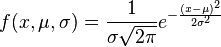
This may look complicated at first, but it's not. The left-hand side says that the normal model is a function (f) of three variables: x, μ, and σ. Which makes sense: we have to plot some value on the vertical (y) axis based on lots of x-values that we plug into our equation, and the shape of our bell curve is going to depend on the mean of the distribution μ (which tells us how far to the right or left on the number line we should slide our bell curve) and the standard deviation σ (which tells us how fat or skinny the bell will be... bigger standard deviation = more dispersion in the distribution = fatter bell curve). When the mean is 0 and the standard deviation is 1, this is referred to as the standard normal model. It looks like this, and was produced by the code below.
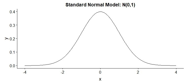
The first line just produces 500 x values for us to work with. The second line creates 500 y values from those x values, produced by the dnorm command (which stands for "density of the normal model"). Because dnorm contains the equation of the normal model, we don't actually have to write out the whole equation. Now we have 500 (x,y) pairs which we can use to plot the standard normal model, using a type of "l" to make it a line, and a line width (using lwd=3) to make it a little thicker (and thus easier to see) than if we used a line width of only one pixel. The z-score tells us how many standard deviations above or below the mean a particular x-value is. You can calculate the z-score for any one of your x-values like this:

The z-score describes what the difference is between your data point (x) and the mean of the distribution (μ), scaled by how skinny or fat the bell curve is (σ). The z-score of the mean of your distribution, then, will be zero - because if x equals the mean, x - μ will be zero and the z-score will be zero. So, ALWAYS:
Positive z-scores are associated with data points that are ABOVE the mean
Negative z-scores are associated with data points that are BELOW the mean
Consider an example where we're thinking about the distribution of several certification exam scores: the ASQ Certified Six Sigma Black Belt (CSSBB) exam from December 2014. Let's say, hypothetically, that we know the population of all scores for this exam can be described by the normal model with a mean of 78 and a standard deviation of 5:

There are a LOT of things we know about the test scores simply by knowing what model represents the data. For example:
The test score that is one standard deviation below the mean is 73 (which we get by taking the mean, 78, and subtracting one standard deviation of 5). This test score of x=73 corresponds to a z-score of -1.
The test score that is one standard deviation above the mean is 83 (which we get by taking the mean, 78, and adding one standard deviation of 5). This test score of x=83 corresponds to a z-score of +1.
The test score that is two standard deviations below the mean is 68 (which we get by taking the mean, 78, and subtracting two times the standard deviation of 5, which is 10). This test score of x=68 corresponds to a z-score of -2.
The test score that is two standard deviations above the mean is 88 (which we get by taking the mean, 78, and adding two times the standard deviation of 5, which is 10). This test score of x=88 corresponds to a z-score of +2.
The test score that is three standard deviations below the mean is 63 (which we get by taking the mean, 78, and subtracting three times the standard deviation of 5, which is 15). This test score of x=63 corresponds to a z-score of -3.
The test score that is three standard deviations above the mean is 93 (which we get by taking the mean, 78, and adding three times the standard deviation of 5, which is 15). This test score of x=93 corresponds to a z-score of +3.
Let's say YOU scored an 85. (There's no way to actually know this, because the certification administrators don't reveal any information about the CSSBB exam beyond whether you passed it or not.) What's your z-score? It's easy to calculate:

A z-score of +1.4 means that your test score was 1.4 standard deviations above the mean of 78. There is also other information that we can find out by knowing what normal model represents the scores of all test-takers.
For example, we know that a very tiny portion of the test-takers (in fact, only 0.3%) scored either above a 93, or below a 63. We can also show that your score of 85% was better than 91.9% of all test-takers. But how??
The 68-95-99.7 Rule
The area under the normal curve reflects the probability that an observation will fall within a particular interval. Area = Probability! There are a couple simple things that you can memorize about the normal model that will help you double-check any problem solving you do with it. Called the empirical rule, this will help you remember how much of the area under the bell curve falls between different z-scores. First, think about how the normal model is symmetric... if you fold it in half (from left to right) at the mean, the curve is a mirror image of itself. The right half of the bell is exactly the same shape and size as the left half. (The code to produce these charts is below the images.)
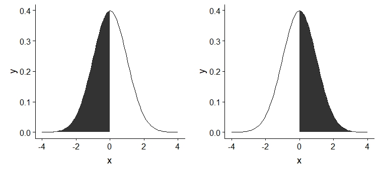
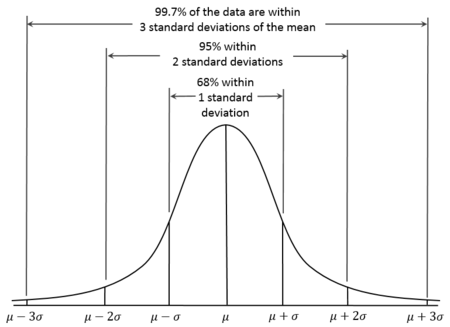
Because the total area under the normal curve is 100%, this also means that 50% of the area under the curve is to the left of the mean, and the remaining 50% of the area under the curve is to the right of the mean. The 68-95-99.7 Empirical Rule provides even more information:
68% of your observations will fall between one standard deviation below the mean (where z = -1) and one standard deviation above the mean (where z = +1)
95% of your observations will fall between two standard deviations below the mean (where z = -2) and two standard deviations above the mean (where z = +2)
99.7% (or pretty much ALL!) of your observations will fall between three standard deviations below the mean (z = -3) and three sd’s above the mean (where z = +3).
Here's what those areas look like. You read "P[-1 < z < 1]" as "the probability that the z-score will fall between -1 and +1".
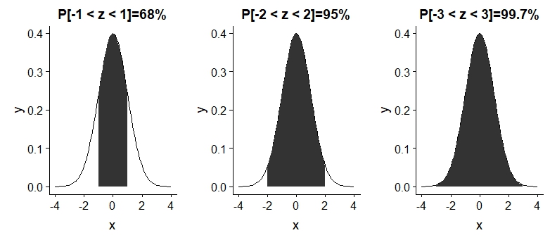
These graphs show that:
There is a probability of 68% that an observation will fall between one standard deviation below the mean (where z = -1) and one standard deviation above the mean (where z = +1).
There is a probability of 95% that an observation will fall between two standard deviations below the mean (where z = -2) and two standard deviations above the mean (where z = +2)
There is a probability of 99.7% that an observation will fall between three standard deviations below the mean (where z = -3) and three standard deviations above the mean (where z = +3)
When data are distributed normally, there is only a VERY TINY (0.3%!) chance that an observation will be smaller than whatever value is three standard deviations below the mean, or larger than three standard deviations above the mean! Nearly all values will be within three standard deviations of the mean. That's one of the reasons why you can use the z-score for a particular data point to figure out just how common or uncommon that value is.
The chart for the 68-95-99.7 rule as presented on Wikipedia is shown on the next page (it's from http://en.wikipedia.org/wiki/68%E2%80%9395%E2%80%9399.7_rule). From the 68-95-99.7 rule, we can estimate what proportion of the population will have scored below our certification score of 85, compared to the normal model with the mean of 78 and the standard deviation of 5, or N(78,5).
The 68-95-99.7 Rule is Great, But Prove it to Me
When you integrate a function, you are computing the area under the curve. So, if we integrate the equation for the normal model between z=-1 and z=+1, we should get an area of 68%. Let's do that. First, we start with the equation of the normal probability distribution function:
Then simplify it using the standard normal model of N(0,1) which is centered at a mean (μ) of 0, with a standard deviation (σ) of 1. (This just means plug in 0 for μ and 1 for σ.) You get:
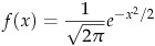
Now, let's integrate it from a z-score of -1 to a z-score of +1 to find the area between those left and right boundaries. We can pull the first fraction outside the integral since it's a constant:
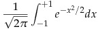
How do we integrate this expression? My lazy solution (since I'm not a mathematician) is to look at a table of integrals, or use Wolfram Alpha at http://www.wolframalpha.com. All we need to do is figure out how to evaluate the stuff on the right side of the integral, then multiply it by one over the square root of 2π. I'll show you what I typed into Wolfram to make it determine the integral for me:
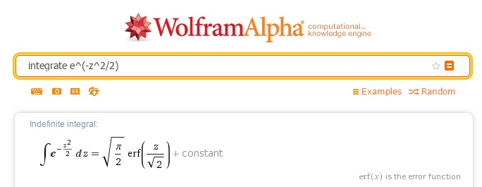
The evaluated integral contains something called erf, the "error function". This is a special function that (fortunately) Wolfram knows how to evaluate as well. Let's plug the result from evaluating this integral back into our most recent expression. That vertical bar on the right-hand side means "evaluate the error function of x over the square root of 2 using x=1, then subtract off whatever you get when you evaluate the error function of x over the square root of 2 using x=-1".
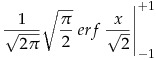
We can simplify all the stuff on the left-hand side of erf because they are all constants... it reduces to a very nice and clean 1/2. So we just need to take the difference between evaluating the error function at x=1, and evaluating the error function at x=-1, and then chop it in half to get our answer. Wolfram will help:
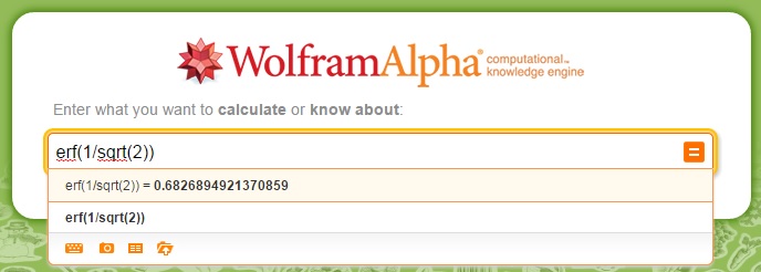
All we had to do was type in erf(1/sqrt(2)) and Wolfram evaluates the right hand side of our expression at x=1, giving us approximately 0.683. If we do this again using x=-1, we'll get a value of -0.683. Now let's plug it all in together:

The area under the standard normal curve between -1 and +1 is 0.683, or 68.3%... nearly the same value that we get from our "rule of thumb" 68-95-99.7% rule! You can try this same process to determine the area under the normal between -2 and +2, or between -3 and +3, to further confirm the empirical 68-95-99.7% rule for yourself.
Calculating All of the Z-Scores for a Data Set
There may come a time where you would like to easily compute the z-scores for each element in a data set that's normally (or nearly normally) distributed. You could take each value individually and use this equation to compute the z-scores one by one:

Or you could just enter your data set into R:
And then have it compute all the z-scores for you at once, using the scale command:
Do these values make sense? Let's check. The mean of our test scores is around 78, so all the scores above 78 should have positive z-scores, and all the scores below 78 should have negative z-scores. We see by examining the original data that scores 1, 2, 3, 6, 8, and 10 are all above the mean, and so should have z-scores that are positive. The output from scale confirms this expectation. We can also see that the third value of 78.5 is just slightly above the mean, so its z-score should be very tiny and positive. It is, at 0.0333.
Using the Normal Model to Answer Questions About a Population
For this collection of examples, we'll use real exam scores from a test I administered last year. You can get my CSV-formatted data directly from GitHub as long as you have the appropriate URL:
If the code above has successfully found and retrieved the data, you should be able to see the semester when the students took the test (in the when variable) and the raw scores (stored in the score variable) when you display the tibble. There are 96 observations in this dataset, the score is a number (of type double), and the semester is a factor (categorical variable) with three levels:
# A tibble: 96 x 2
when score
<fct> <dbl>
1 FA14 45.0
2 FA14 55.0
3 FA14 42.5
4 FA14 37.5
5 FA14 30.0
6 FA14 47.5
7 FA14 40.0
8 FA14 45.0
9 FA14 32.5
10 FA14 47.5
# ... with 86 more rows
First, we should check and see whether the scores are approximately normally distributed. We can do this by plotting a histogram, then by doing a QQ plot which (if are scores are nearly normal) should show all of our data points nearly along the diagonal. QQ plots and tests for normality are covered more extensively in Chapter 2.8.
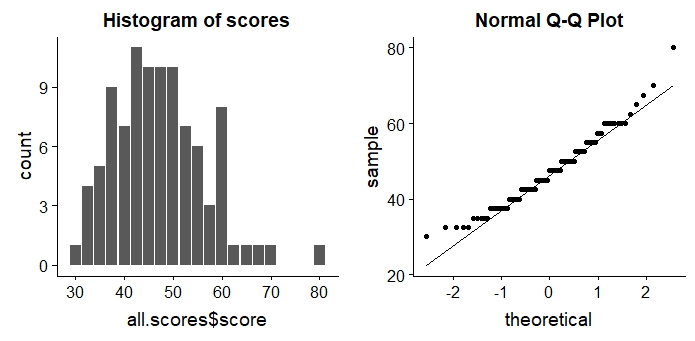
The histogram is skewed a little to the right, but it's nearly normal, so we can proceed. To figure out what normal model can be used to represent the data, we need to know the mean and standard deviation of the scores:
# A tibble: 1 x 1
mean
<dbl>
1.  47.3
# A tibble: 1 x 1
sd
<dbl>
1 9.31Rounding a bit, we should be able to use N(47.3,9.3) (or "the normal model with a mean of 47.3 and a standard deviation of 9.3") to represent the distribution of all our scores. Using this model, we can answer a lot of questions about what the population of test-takers looks like. Looking at the histogram, we can see that a score of 50 is about in the middle. What proportion of students got below a 50? We can answer this question by determining the area under N(47.3,9.3) to the LEFT of x=50 (x<50 in code). It looks like this:
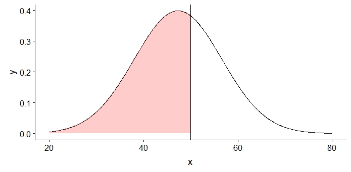
Here’s the code that produced this plot:
Here’s a comparable base R way to get the same-ish plot:
Since the mean is 47.3, we know that a test score of 50 is TO THE RIGHT OF THE MEAN. The z-score associated with 50 is going to be positive. How positive will it be? Well, since the standard deviation is 9.3, we know that the test score which is one standard deviation above the mean will be 47.3 + 9.3 = 56.6. Our test score of 50 is just a little bit above the mean, so we can estimate our z-score at +0.3 or +0.4. That means the area under the normal to the left of x=50 will be greater than 50%, but not much greater than 50%. Even before we do the problem, we can estimate that our answer should be between 55% and 65%.
To definitively determine the area below the curve to the left of x=50, we use the pnorm function in R. The pnorm function ALWAYS tells us the area under the normal curve to the LEFT of a particular x value (remember this!!) So we can ask it to tell us the area to the left of x=50, given a normal model of N(47.3,9.3):
We can predict that 61.4% of the test-takers in the population received a score less than 50%. This means even though our data set only includes students from a couple of semesters of my class, we've found a way to use this sample to determine what the scores from the entire population of students who took this test must be! As long as my students are representative of the larger population, this should be a pretty good bet. (What if you don't have R? Don’t worry, you can still use Z Score Tables or online Z Score Calculators to find the area under the normal curve. Z Score Tables are in the back of most statistics textbooks. Let's do the same problem we just did, AGAIN, using tables and calculators.)
Let's do this problem with a Z Score Table. First Rule of Thumb: ALWAYS PICK A Z SCORE TABLE THAT HAS A PICTURE OF THE NORMAL CURVE ON IT.
http://www.stat.ufl.edu/~athienit/Tables/Ztable.pdf HAS a picture. Use this kind!
http://www.utdallas.edu/dept/abp/zscoretable.pdf DOES NOT HAVE a picture. DO NOT USE this kind of table!
It's best to use Z Score Tables that have pictures so you can match the picture representing the area under the curve you're trying to find with the picture. To find the area under the curve, you need a z-score. The z-score that corresponds with a test score of x=50 is

When we look at the picture we drew, notice that the shaded portion is bigger than 50% of the total area under the curve. When we look at the picture in the Z Score Table from http://www.stat.ufl.edu/~athienit/Tables/Ztable.pdf, it does NOT look like what we drew:
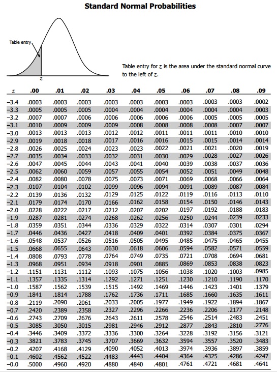
This particular Z Score Table ONLY contains areas within the tails. The trick to using a Z Score Table like this is to recognize that because the normal distribution is symmetric, the area to the LEFT of z=+0.29 can be found by taking 100% of the area, and subtracting the area to the LEFT of the z-score at z=-0.29 (what's in the area of the tail). Using the Z Score Table from http://www.stat.ufl.edu/~athienit/Tables/Ztable.pdf, we look in the row containing z=-0.2, and the column containing .09, because these add up to our computed z-score of 0.29. We get an area of 0.3859. But we're looking for an area greater than 50% (which we know because we drew a PICTURE!), so we take 1 - 0.3859 to get 0.6141, or 61.4%.
Let's say we don't have a Z Score Table handy, and we don't have R. What are we to do? You can look online for a Z Score Calculator which should also give you the same answer. I always use Wolfram. There are so many Z Score Calculators out there... and only about half of them will give you the right answers. It's really sad! But Wolfram will give you the right answer, and it also asks you to specify what area you're looking for using very specific terminology. I can ask Wolfram "What's the area under the normal curve to the left of z=0.29?" like this:
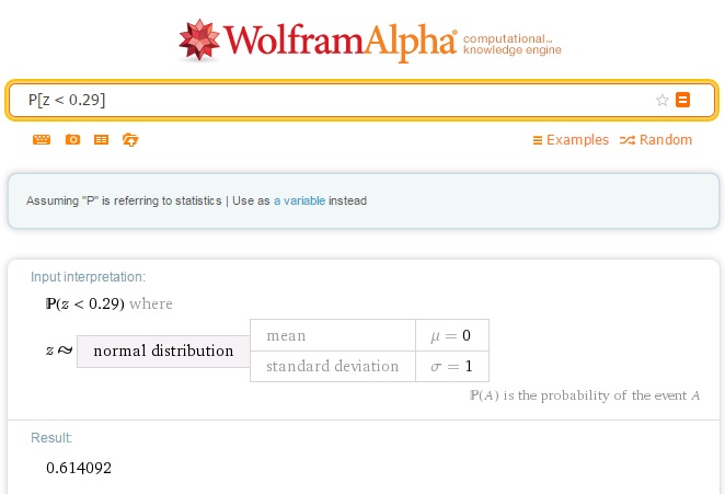
The area is 0.614, or 61.4% - the same as we got from the Z Score Table and the pnorm calculation in R.
Let's Do Another Z Score Problem
Say, instead, we wanted to figure out what proportion of our students scored between 40 and 60. That means we want to find the area under N(47.4, 9.3) between x=40 and x=60. For these examples, we will continue to use ggplot with geom_vline to drop the vertical lines, and geom_area to shade under the curve:
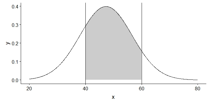
To calculate this area, we'll have to take all the area to the left of 60 and subtract off all the area to the left of 40, because pnorm and Z Score Calculators don't let us figure out "areas in between two z values" directly. So let's do that. Graphically, we'll take the total area in the left graph below, and subtract off the area of the right graph in the middle, which will leave us with the area in the graph on the right:
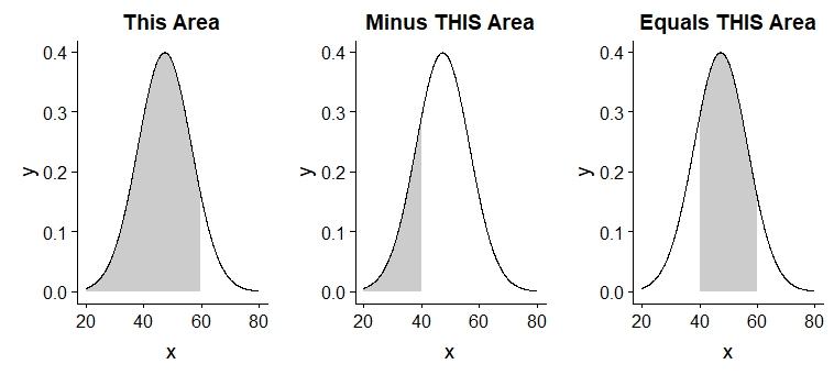
labels <- c("This Area", "Minus THIS Area", "Equals THIS Area")
Fortunately, we can look up areas under the normal curve very easily with the pnorm command in R. We’ll do it using two terms. The first term (to the left of the minus sign) finds all of the area to the left of x=60, and the second term (to the right of the minus sign) finds all of the area to the left of x=40. We subtract them to find the area in between:
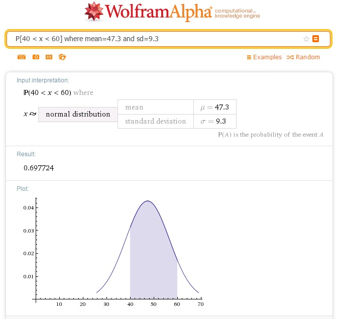
We can also do this in Wolfram as long as we know how to ask for the answer (see next page). All of the methods give us the same answer: 69.7% of all the test scores are between x=40 and x=60. I would really have preferred that my class did better than this! Fortunately, these scores are from a pre-test taken at the beginning of the semester, which means this represents the knowledge about statistics that they come to me with. Looks like I had a completely green field of minds in front of me... not a bad thing.
Let's Go Back to That Problem from the Beginning
So in the beginning of the chapter, we were talking about an example where WE scored an 85 on a certification exam where all of the test scores were normally distributed with N(78,5). Clearly we did well, but we want to know: what percentage of all test-takers did we score higher than? Now that we know about pnorm, this is easy to figure out, by drawing and shading under the normal curve and sending the right arguments to pnorm:
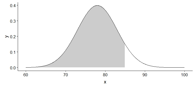
From the picture, we can see that we scored higher than at least half of all the test-takers. Using pnorm, we can tell exactly what the area underneath the curve is:
Want to double check? Calculate the z-score associated with 85 for this particular normal distribution, head to Wolfram, and ask it to calculate P[z < whatever z score you calculated].
You Don't Need All the Data
In the examples above, we figured out what normal model to use based on the characteristics of our data set. However, sometimes, you might just be told what the characteristics of the population are - and asked to figure out what proportion of the population has values that fall above, below, or between certain outcomes. For example, let's say we are responsible for buying manufactured parts from one of our suppliers, to use in assemblies that we sell to our customers. To work in our assembly, each part has to be within 0.01 inches of the target length of 3.0 inches. If our supplier tells us that the population of their parts has a mean length of 3.0 inches with a standard deviation of 0.005 inches, what proportion of the parts that we buy can we expect to not be able to use? (This has implications for how many parts we order, and what price we will negotiate with our supplier.)
To solve this problem, we need to draw a picture. We know that the length of the parts is distributed as N(3.0, 0.005). We can't use parts that are shorter than (3.0 - 0.01 = 2.99 inches), nor can we use parts that are longer than (3.0 + 0.01 = 3.01 inches):
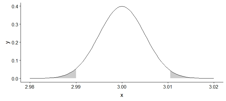
What proportion of the area is contained within these tails, which represent the proportion of parts we won't be able to use? Because the normal model is symmetric, as long as we can find the area under the curve inside one of those tails, we can just multiply what we get by two to get the area in both of the tails together.
Since pnorm always gives us the area to the left of a certain point, let's use it to find out the area in the left tail. First, let's calculate a z score for x=2.99:

Using the 68-95-99.7 rule, we know the area we're looking for will be about 5% (since 95% of the area is contained inside z=-2 and z=+2). Let's look up to see what the area is exactly, multiplying by 2 since we need to include the area in both tails:
We can also ask pnorm for the area directly, without having to compute the z score. Notice how we give pnorm the x value at the boundary of the left tail, since we know pnorm gives us everything to the left of a particular x value:
All methods agree. Approximately 4.5% of the parts that we order won't be within our required specifications. If this was a real problem we were solving for our employer, though, the hard part would be yet to come: how are we going to use this knowledge? Does it still make sense to buy our parts from this supplier, or would we be better off considering other alternatives? Should we negotiate a price discount? Solving problems in statistics can be useful, but sometimes the bigger problem comes after you've done the calculations.
Now What?
My favorite picture of z-scores superimposed on the normal model is here. Print it out! Carry it with you! Memorize it! http://en.wikipedia.org/wiki/Standard_score
If you want to know more about the normal model, Wolfram has an excellent page that goes into depth at http://mathworld.wolfram.com/NormalDistribution.html
Notice that in all the examples from this chapter, we know details about the population. If we're only able to select a small sample of items from our population (usually less than 30), we aren't going to be able to get a really good sense of the variability within the population. We have to adjust our normal model to account for the fact that we only have limited knowledge of the variability within the population: to do that, we use the t distribution.