1.6 Getting Data Into R
Objectives
Before you can manipulate and analyze data, first you have to load it into R. The purpose of this section is to introduce you to techniques for acquiring data and manipulating data structures in R. You will:
Learn how to get, set, and explore working directories with getwd and setwd
Learn how to open a file on your local machine using read.csv and read.table
Learn how to retrieve data that is accessible on the web using a URL
Learn how to retrieve data that is stored in spreadsheet format on Google Docs (using Jenny Bryan’s amazing googledocs package)
Inspect data using head, tail, and str
Understand why it's important to be aware of data types and data structures as you're acquiring data from different kinds of sources
Step 1: Getting, Setting, and Viewing Contents of the Working Directory
The concept of the working directory is fundamental to R. Basically, R can only be pointing to (and looking at) one directory on your machine at any given time. Much of the time, your data will be stored on your local machine, and you need to load it into R so you can manipulate and analyze it. If you want to find out which directory R is looking at right now, "get your working directory" by typing getwd() - I’ll show you what it looks like when I do it on my machine:
When you execute this command on your machine, you may or may not be pointed to the same directory that’s displayed above. The first step will be to tell R where you want it to look for datasets. I have a “work in progress” directory called R on my D drive where I keep some datasets, so that’s the location I want to “set my working directory” to:
setwd("D:/R")Then, you can find out what's in that directory by typing dir():
The displayed files are stored as a data frame, so you can capture these values and use them in your programming later. For example, let’s do this using a variable called my.dir:
Once you know where your data is located, there are many methods to import it into R:
If your data is stored as TXT, CSV, or XLS and listed in the directory contents displayed on your screen, go to Step 2 Option A to import it into R,
If your data is online as a Google Spreadsheet, go to Step 2 Option B
If your data is on GitHub, go to Step 2 Option C
If your data is online but at another URL, go to Step 2 Option D
If you just want to use R’s built-in data sets, go to Step 2 Option E
If you want to load JSON data, go to Step 2 Option F
…and follow the instructions. I tend to store and retrieve my data as CSV (comma-separated variables) files, and keep notes in TXT format. I do data entry, editing, and cleaning in Excel, but then save the contents as CSV for import into R. Everyone has different preferences.
Step 2 Option A: Loading Data from a TXT, CSV, or XLS file on Your Machine
When you first install the base R package, you are provided with several rudimentary commands to import data, including read.table (to bring in observations that are separated by spaces or tabs) and read.csv (to bring in observations that are separated by commas). I have a text file with data in it called x.txt that contains observations of M&M candies. If I open the file with a text editor, the variable names are in the first row, and the observations are in subsequent rows:
student id color defect hour minute weight total.number
1 1 1 2 10 48 50.14 57
1 12 1 4 10 49 50.14 57
1 23 1 2 10 49 50.14 57
1 34 1 4 10 49 50.14 57
1 45 1 4 10 50 50.14 57
30 34 1 4 10 42 48.3 49
30 3 1 4 10 44 48.3 49
Because the observations are separated by tabs, the columns do not appear aligned in the text editor, but R will know which observations correspond to which variables. Use read.table() to import the data, use head() to make sure it’s been imported correctly, and use str() to see what variable types are contained in the dataset. We use header=TRUE to declare that the first row of our file contains variable names.
my.data <- read.table("x.txt",header=TRUE)
head(my.data)
student id color defect hour minute weight total.number
1 1 1 1 2 10 48 50.14 57
2 1 12 1 4 10 49 50.14 57
3 1 23 1 2 10 49 50.14 57
4 1 34 1 4 10 49 50.14 57
5 1 45 1 4 10 50 50.14 57
6 30 34 1 4 10 42 48.30 49str(my.data)'data.frame': 2884 obs. of 8 variables:
$ student : int 1 1 1 1 1 30 30 30 30 30 ...
$ id : int 1 12 23 34 45 34 3 10 22 43 ...
$ color : int 1 1 1 1 1 1 1 1 1 1 ...
$ defect : int 2 4 2 4 4 4 4 2 4 4 ...
$ hour : int 10 10 10 10 10 10 10 10 10 10 ...
$ minute : int 48 49 49 49 50 42 44 46 49 51 ...
$ weight : num 50.1 50.1 50.1 50.1 50.1 ...
$ total.number: int 57 57 57 57 57 49 49 49 49 49 ...
Importing data from CSV is very similar, only the raw data is separated by commas:
"sg","V1","V2","V3","V4"
"sg1",1.397,1.349,1.278,1.279
"sg2",1.397,1.399,1.397,1.311
"sg3",1.397,1.288,1.29,1.828
This data is contained in a file called xbar-r-subgroups.csv which is a tiny file that contains data I collected while starting a control chart exercise. We use read.csv() to pull it into a variable called cc.data (for “control chart data”) in R:
cc.data <- read.csv("xbar-r-subgroups.csv",header=TRUE)
head(cc.data)
sg V1 V2 V3 V4
1 sg1 1.397 1.349 1.278 1.279
2 sg2 1.397 1.399 1.397 1.311
3 sg3 1.397 1.288 1.290 1.828str(cc.data)'data.frame': 3 obs. of 5 variables:
$ sg: Factor w/ 3 levels "sg1","sg2","sg3": 1 2 3
$ V1: num 1.4 1.4 1.4
$ V2: num 1.35 1.4 1.29
$ V3: num 1.28 1.4 1.29
$ V4: num 1.28 1.31 1.83
To load an Excel file like this one, you have to obtain the xlsx package first:
library(xlsx)Fortunately, the process for importing is identical to the previous two methods. Just use read.xlsx instead of read.table, read.csv, or read_csv. [Note: The xlsx package depends on the rJava package, which also requires that you have a functioning version of Java on your machine and IN YOUR PATH. If you don’t know what this means, or how to make both of these things happen, then I’d stick to saving your files as CSV or TXT and using the other import methods. I am not providing an example of this because I don’t have Java, rJava, or xlsx installed on my machine, and I try not to use Excel for anything other than data cleaning.
Step 2 Option B: Loading Data from Google Spreadsheets
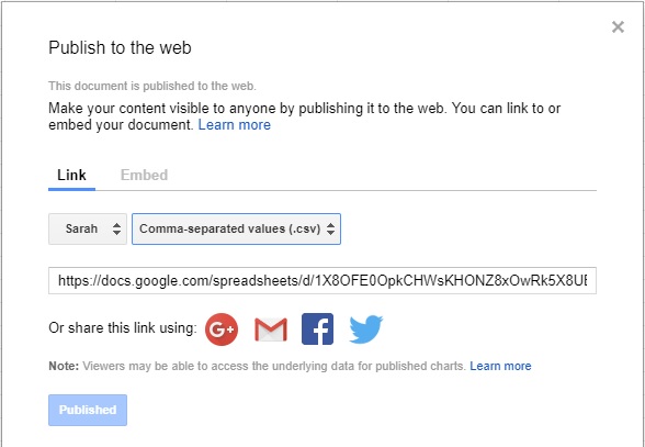
To import data stored in the cloud on Google Spreadsheets, there are three options. The easiest option, if you own the Google Spreadsheet, is to publish the data to the web as a CSV file, and then load it in directly using read_csv. For example, I stored a data set at this long URL (which you should be able to load it up from your R console as well):
# A tibble: 78 x 6
subject equipment task size.cm distance.cm response.time.ms
<chr> <chr> <int> <dbl> <dbl> <int>
1 Sarah PC 1 0.500 1. 965
2 Sarah PC 1 0.500 1. 966
3 Sarah PC 1 0.500 1. 931
4 Kyle PC 1 0.500 1. 953
5 Kyle PC 1 0.500 1. 892
6 Kyle PC 1 0.500 1. 935
7 Troy PC 1 0.500 1. 1063
8 Troy PC 1 0.500 1. 1005
9 Troy PC 1 0.500 1. 1483
10 Sarah VR 1 0.500 1. 1288
# ... with 68 more rows
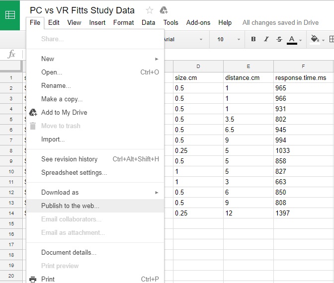
Publishing data to the web is a two-step process. First, go to File -> Publish to the Web. This will take you to a second screen where you will choose which spreadsheet to publish, and the target format (CSV):
The second option is to open the data in Google Drive and download a copy of it to your local machine. You do this by going to
File -> Download As -> Comma-separated values (.csv, current sheet)
Remember what directory you used to store the file, because you will need to make sure you set your R working directory to that location before using read.csv to import.
Your third option is to use Jenny Bryan’s googlesheets package. First download and wake it up in R, using the dependencies=TRUE argument which will also download the additional packages this one depends on:
library(googlesheets)I want to load the M&M data that’s in the Google sheet at this URL. Paste it into your address bar so you can see the data:
https://docs.google.com/spreadsheets/d/1tykXpknyrpu25Z6kWM55iVxKihV2ZkLhuj4ZDyCV7w8/
We need to know the DOCUMENT KEY to pull this data into R. This is the long, unintelligible sequence of letters and numbers in the URL after you see “/d/”. The first thing we have to do in R is to create a variable to store this document key:
Next, we make a connection between R and this googlesheet:
my.gs <- gs_key(ss.key)Finally, we can use that connection to import the data and create a data frame called mnms in R. If it works, you should see indications of progress displayed:
mnms <- as.data.frame(gs_read(my.gs))Accessing worksheet titled 'Sheet1'.
Downloading: 4.3 kB Downloading: 4.3 kB Downloading: 12 kB Downloading: 12 kB Downloading: 13 kB Downloading: 13 kB Downloading: 13 kB Downloading: 13 kB No encoding supplied: defaulting to UTF-8.
Warning: 1 parsing failure.
row col expected actual
1402 id an integer C
Warning message:
Missing column names filled in: 'X9' [9]
Finally, use the head command to make sure the data actually showed up.
head(mnms)student id color defect hour minute weight total.number X9
1 allenrj 1 BL L 10 48 50.14 57 NA
2 allenrj 2 BL N 10 49 50.14 57 NA
3 allenrj 3 BL L 10 49 50.14 57 NA
4 allenrj 4 BL N 10 49 50.14 57 NA
5 allenrj 5 BL N 10 50 50.14 57 NA
6 Pinoja 4 BL N 10 42 48.30 49 NA[Note 1: Even though it seems like you might be able to simplify the import code, for example by encoding the document key directly inside the gs_key command, or maybe by mashing them all together instead of having them on separate lines… it doesn’t usually work.]
[Note 2: Sometimes, security issues prevent the googlesheets commands from working. If you are having problems, try typing this to authenticate: my_sheets <- gs_ls() ]
Step 2 Option C: Loading Data from GitHub
In addition to being an excellent environment for source code configuration management, GitHub (http://github.com) is also a place where you can store changing versions of datasets. All of the data that I use for examples in my books can be found in my GitHub data directory at https://github.com/NicoleRadziwill/Data-for-R-Examples. We will load in a CSV file and a plain text file as examples. First, you need to find the URL that corresponds to the raw data by drilling down into the file you want to obtain, and then clicking the “Raw” button on the right-hand side of the page. If I drill down into comp-temps.csv (which contains three months of temperature observations from two recording stations in Virginia), the URL that appears is https://raw.githubusercontent.com/NicoleRadziwill/Data-for-R-Examples/master/comp-temps.csv.
You can cut and paste this URL into the address bar to see the data yourself. Next, obtain the data like this. The head command displays the first six rows, so you can make sure it imported correctly:
id date cho shd diff
1 1 20140601 75 73 2
2 2 20140602 81 80 1
3 3 20140603 83 81 2
4 4 20140604 88 84 4
5 5 20140605 81 78 3
6 6 20140606 81 77 4
You can also do it in one line by replacing your file name, in quotes, within read.csv() – but I like to create a new variable to store my URL to make my code cleaner and easier later, if (and when) I have to reload my data or start a new R session.
Step 2 Option D: Loading Data from a URL
Perhaps your data is stored on the web somewhere (like in the UCI Machine Learning Repository at http://archive.ics.uci.edu/ml/datasets.html), and you can see it in your web browser and want to get it into R. Load it in directly:
# A tibble: 208 x 10
adviser \`32/60\` \`125\` \`256\` \`6000\` \`256_1\` \`16\` \`128\`
\`198\` \`199\`
<chr> <chr> <int> <int> <int> <int> <int> <int> <int>
<int>
1 amdahl 470v/7 29 8000 32000 32 8 32 269 253
2 amdahl 470v/7a 29 8000 32000 32 8 32 220 253
3 amdahl 470v/7b 29 8000 32000 32 8 32 172 253
4 amdahl 470v/7c 29 8000 16000 32 8 16 132 132
5 amdahl 470v/b 26 8000 32000 64 8 32 318 290
6 amdahl 580-5840 23 16000 32000 64 16 32 367 381
7 amdahl 580-5850 23 16000 32000 64 16 32 489 381
8 amdahl 580-5860 23 16000 64000 64 16 32 636 749
9 amdahl 580-5880 23 32000 64000 128 32 64 1144 1238
10 apollo dn320 400 1000 3000 0 1 2 38 23
# ... with 198 more rows
Step 2 Option E: Using One of R’s Canned Datasets
If you just want to try out some of the techniques in this book, you might not want to go through the struggle of collecting, recording, cleaning, or simulating data. Fortunately, R has hundreds of built-in datasets that you can use. Not all of these datasets are created equal. In fact, basically none of them have identical data structures, so it is extremely important to inspect the data (Step 3) before you try anything interesting. For example, to get Edgar Anderson’s famous iris data, do this:
Sepal.Length Sepal.Width Petal.Length Petal.Width Species
1 5.1 3.5 1.4 0.2 setosa
2 4.9 3.0 1.4 0.2 setosa
3 4.7 3.2 1.3 0.2 setosa
4 4.6 3.1 1.5 0.2 setosa
5 5.0 3.6 1.4 0.2 setosa
6 5.4 3.9 1.7 0.4 setosa
To see what additional datasets are available, type data().
Inspecting Data with head, tail, and str
Each time we retrieve and import data, it’s important to check and see if it actually showed up in R. The head command, which you’ve seen several times now, returns the first six elements of the data structure (or, for a data frame, the first six rows). The tail command displays the last six:
Sepal.Length Sepal.Width Petal.Length Petal.Width Species
145 6.7 3.3 5.7 2.5 virginica
146 6.7 3.0 5.2 2.3 virginica
147 6.3 2.5 5.0 1.9 virginica
148 6.5 3.0 5.2 2.0 virginica
149 6.2 3.4 5.4 2.3 virginica
150 5.9 3.0 5.1 1.8 virginicatail(mnms)student id color defect hour minute weight total.number X9
2879 boltzjr 37 Y L 11 54 48.53 52 NA
2880 boltzjr 38 Y N 11 54 48.53 52 NA
2881 boltzjr 39 Y N 11 55 48.53 52 NA
2882 boltzjr 40 Y N 11 55 48.53 52 NA
2883 boltzjr 41 Y N 11 55 48.53 52 NA
2884 nicho2nx 5 Y N 11 50 47.34 54 NAThe str command tells us what the structure is of the data we just imported. This includes 1) the data type of each variable in our data structure, and 2) the structure of the container within which our data is sitting. Knowing these structures is important because R commands are written to be compatible with certain structures and data types, but not with others. For example, this tells us that the iris dataset is a data frame (which looks like an Excel spreadsheet) containing 150 observations, and each observation has 5 variables (four of which are numeric or quantitative, and one of which is a Factor, or categorical):
'data.frame': 150 obs. of 5 variables:
$ Sepal.Length: num 5.1 4.9 4.7 4.6 5 5.4 4.6 5 4.4 4.9 ...
$ Sepal.Width : num 3.5 3 3.2 3.1 3.6 3.9 3.4 3.4 2.9 3.1 ...
$ Petal.Length: num 1.4 1.4 1.3 1.5 1.4 1.7 1.4 1.5 1.4 1.5 ...
$ Petal.Width : num 0.2 0.2 0.2 0.2 0.2 0.4 0.3 0.2 0.2 0.1 ...
$ Species : Factor w/ 3 levels "setosa","versicolor",..: 1 1 1 1 ...
The structure is also a critical part of your overall approach and troubleshooting strategy. If your analysis code is not working, the first two questions to ask are:
Has my data been imported correctly (that is, does it exist in R)? (Use head or tail)
Are my data structures what I expect? (Use str)
A more in-depth look at R data structures (vectors, lists, matrices, arrays, and data frames) and the data types that make up those data structures (logical, numeric, integer, complex, character, and raw) is provided in the next chapter.
Step 2 Option F: Accessing Real Repositories with APIs, JSON, and rjson
Often, data is not stored on the web but is accessible from the web. You just have to know how to get it, and how to deal with the data format that you are served. It is not uncommon for organizations to offer access to their databases if you know a little programming. They will publish Application Programming Interfaces (or APIs) that provide you with objects and methods to get to their data. Two common data formats are eXtensible Markup Language (XML) and JavaScript Object Notation (JSON). This section covers the JSON format and how to obtain data in JSON format through the R console, using the rjson package. (You can explore XML on your own, if you like.) Be sure to install rjson first!
This example uses the Weather Underground API which is documented online at http://www.wunderground.com/weather/api/. To use it, you first have to register to gain access and get what's called an "API Key". Services like this often want to make sure that you are a real human, and not just a bot who will overload their system with requests for information.
I used my key to obtain a weather observation from San Francisco, and stored the JSON file on GitHub. You can cut and paste the URL below into a browser address bar, and see what the raw data looks like. To pull it into R, use this two-step process:
json.file <-
"https://raw.githubusercontent.com/NicoleRadziwill/Data-for-R-Examples/master/example.json"
json.data <- fromJSON(paste(readLines(json.file), collapse=""))
str(json.data)
$ response :List of 3
..$ version : chr "0.1"
..$ termsofService: chr
"http://www.wunderground.com/weather/api/d/terms.html"
..$ features :List of 1
.. ..$ conditions: num 1
..The fromJSON command reads input in JSON format and automatically converts it into a data structure that is accessible from within R. This is a complicated data structure that consists of lists embedded within other lists!
Additional Resources
For importing LARGE datasets, use fread in the data.table package.
Although we don’t use it much in this book, you can also import space-delimited or tab-delimited data into R using the read.table command. This works well if you are opening a file on your local machine, or retrieving tabular data from GitHub, or retrieving data that has been published in text format from Google Spreadsheets.
If you use RStudio, selecting “Import Dataset” should be all you need, but more info is at https://thepracticalr.wordpress.com/2017/01/31/importing-data-into-r-part-ii/
The readstata13 package can be used to import data from the Stata package.
For more information about the iris data, and the hundreds of R examples that use this data, search for “iris data in r” in Google. When I did the search, it returned 685,000 results.